 Personal Project · Materials Science
Interactive Iron–Carbon Diagram
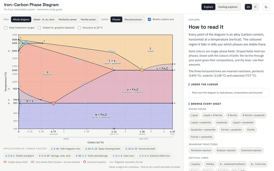
A dense metallurgy chart that you read by pointing at it. Hover over a phase, click for its full sheet, or cool a steel and watch which phases it passes through.
In short
- Problem
- As a flat textbook image, the Fe–Fe₃C diagram is a wall of overlapping fields, Greek letters and invariant points.
- Approach
- Read it by position. Hover for a quick card, click for a full study sheet, or cool a chosen steel and follow the fields and reactions it crosses.
- Result
- A bilingual study tool that runs in the browser, built on reference values for the invariant points, with a broken carbon axis that keeps the steel range readable and the lever rule worked out at any point.
- Tools
- React · SVG
You can try it here. It runs in your browser, in English or Italian, with nothing to install.
Where it came fromLink to this section
I met the iron–carbon diagram in a materials-science course during my bachelor's, and I was struck by how much it packs into one picture. Every region is a phase, every line is a transformation, and every point is a precise composition and temperature at which the structure of the metal changes.
As a flat image on a textbook page, though, it is intimidating. You get a wall of overlapping zones, Greek letters (α, γ, δ) and invariant points, and you're expected to hold all of it in your head at once. Every time I looked at it I had the same thought: this is already a map, so why can't I just point at a place and have it tell me what's there?
The idea: read it by positionLink to this section
That thought became the premise. The diagram's meaning is positional: where you sit on the carbon axis and how hot you are decide everything. So the main interaction had to be positional too. A student shouldn't have to memorise which zone is which. They should be able to move across the diagram and get exactly the information that belongs to the spot they're on.
The metallurgy comes from the textbooks. What I built is the interface: you point at a part of the chart and it tells you what is there.
What it doesLink to this section
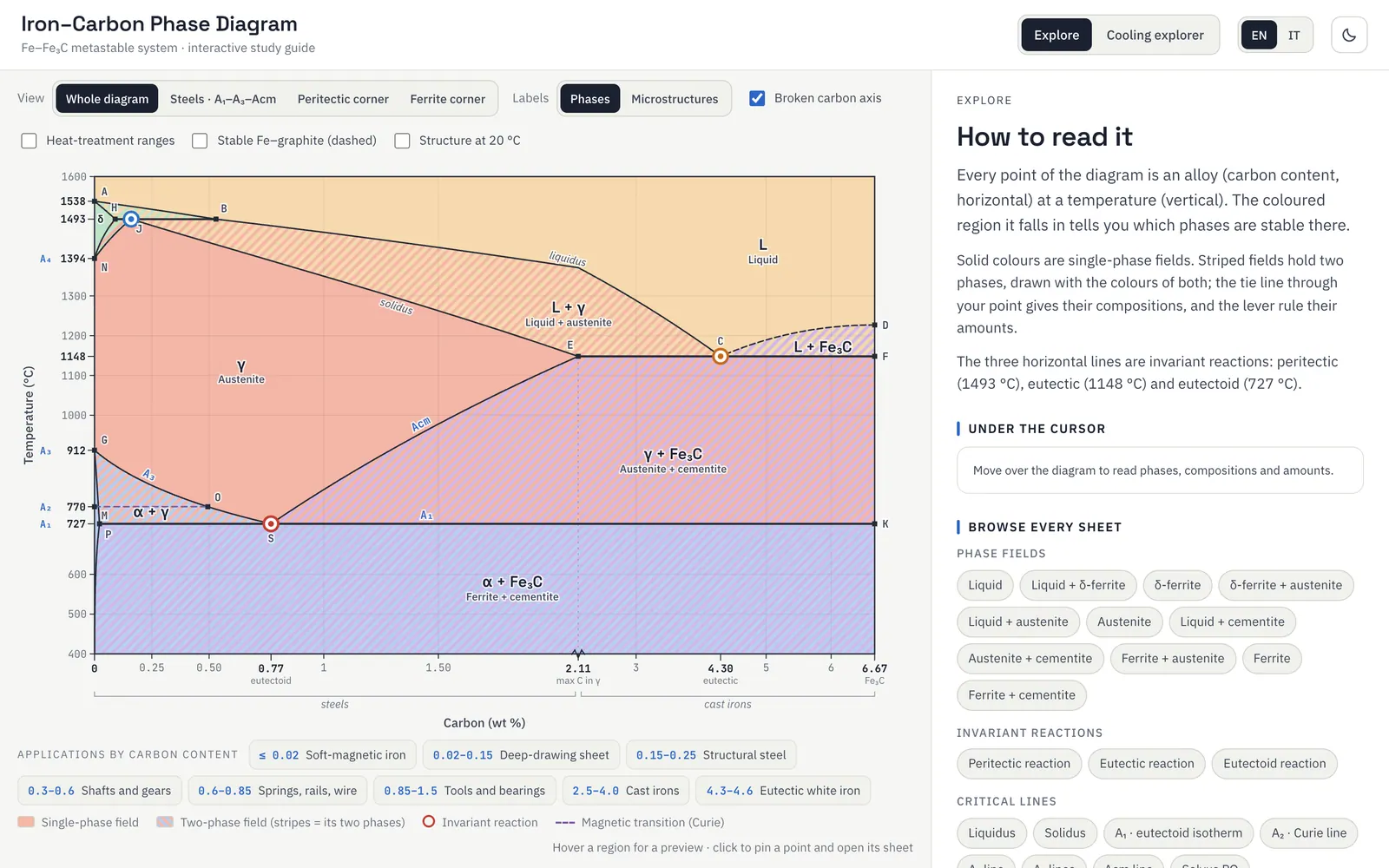
The first layer gives the quick answer. Move over any region and a small card appears with the name of the phase, its composition and temperature range, and a one-line description. There's nothing to click and no menu to open: the information shows up wherever your cursor is.
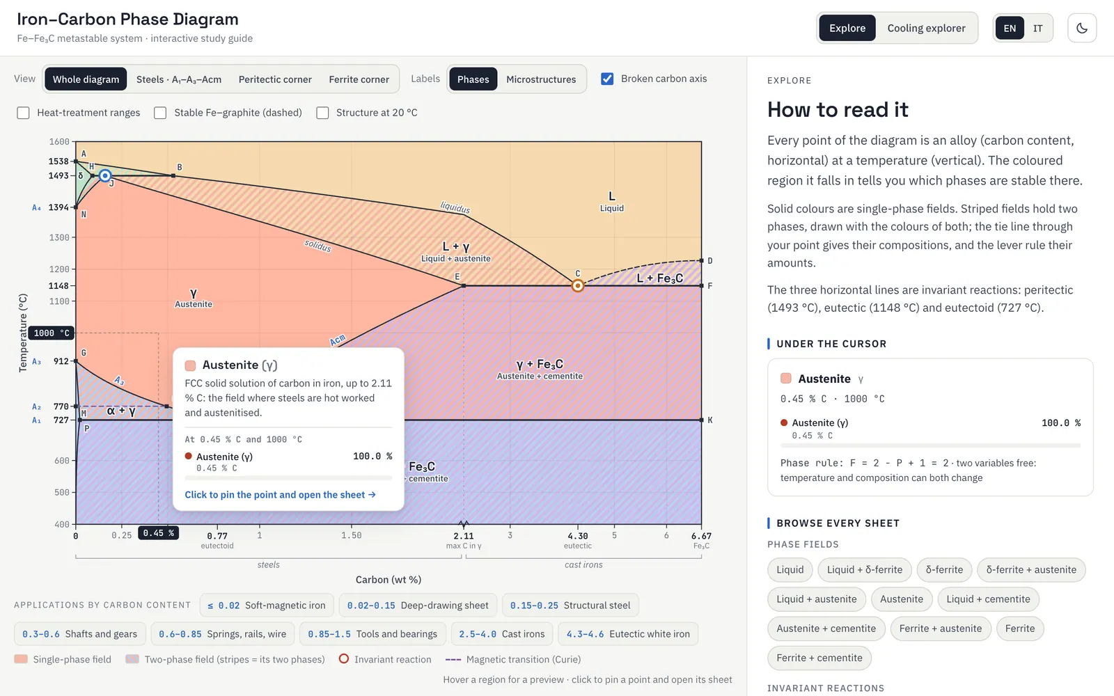
The second layer goes deeper. Click a region or an invariant point and a full study sheet opens next to the diagram. It covers the phases involved, their crystal structures, what physically happens on cooling, the mechanical behaviour that results and the typical applications. Sheets also show drawings of the unit cells and schematic microstructures. If you click inside a two-phase field, the point stays pinned and the sheet works out the lever rule there, with the tie line, the phase compositions and their amounts. Every region, line and point has its own sheet, so what you read always matches where you clicked.
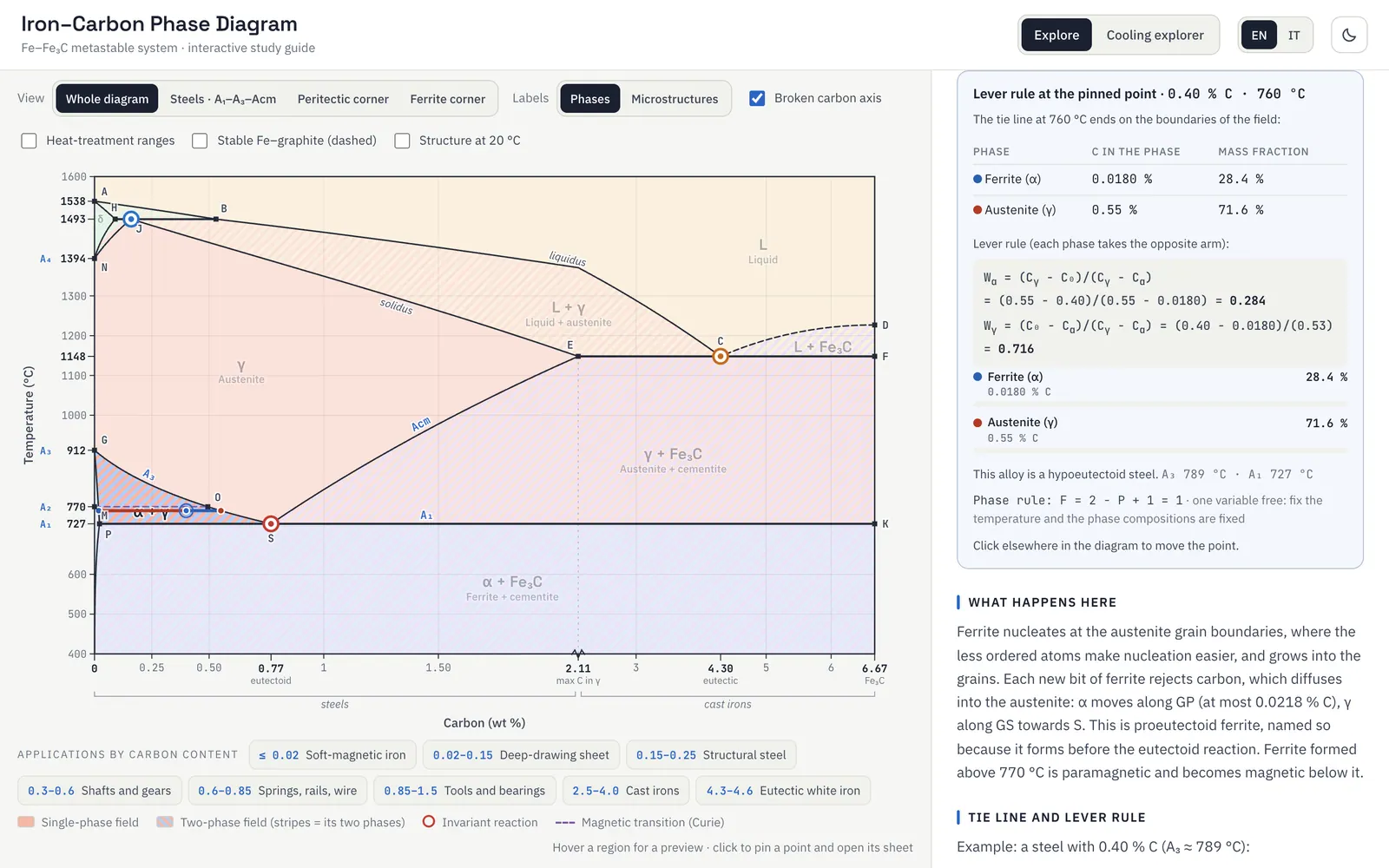
Wγ = 1 − Wα = 0.716
lever rule at the pinned point · 0.40 % C, 760 °C
C₀ is the alloy; Cα and Cγ are the two ends of the tie line at that temperature. Each phase takes the arm on the opposite side of the alloy, and the two fractions add up to 1.
Following a cooling pathLink to this section
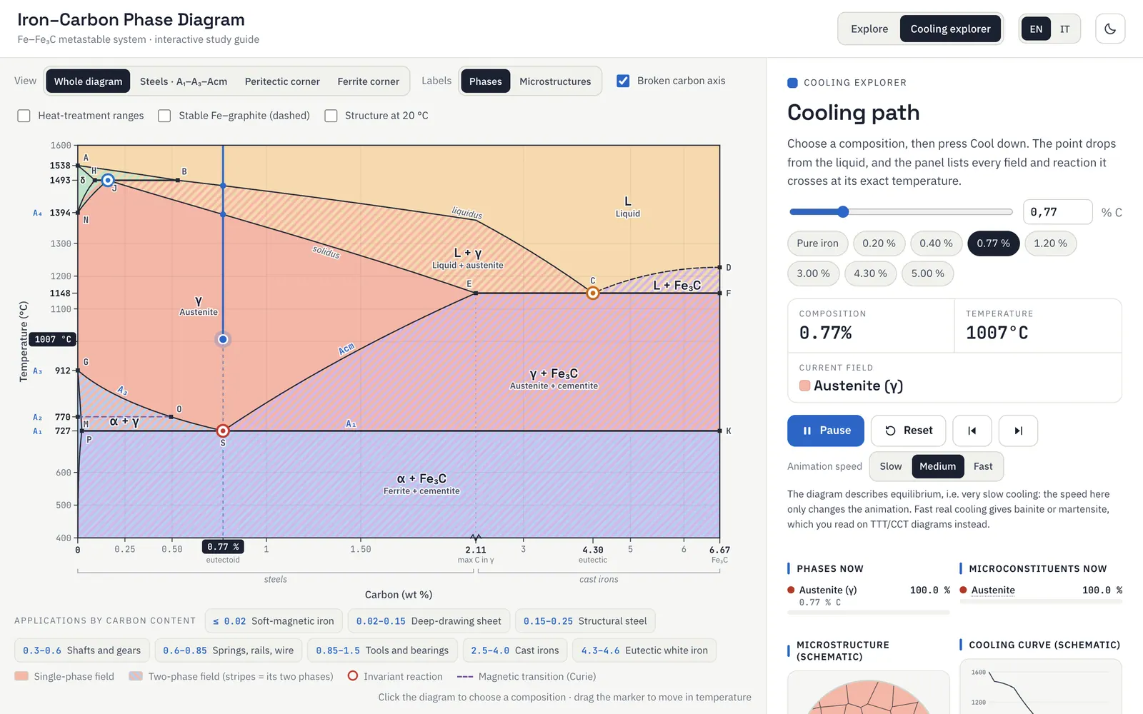
The feature I cared about most answers the question every exercise ends up asking: if I take a steel with a given carbon content and cool it, what does it actually pass through before it becomes the final product? In the cooling explorer you pick a composition and press Cool down. A marker then moves down the temperature axis in real time and tells you which phase field you're in at each moment. Meanwhile the panel builds, from top to bottom, the full list of fields it crosses and the invariant reactions it triggers. Next to it, a schematic micrograph changes grain by grain and a cooling curve shows where the temperature stops while a reaction runs.
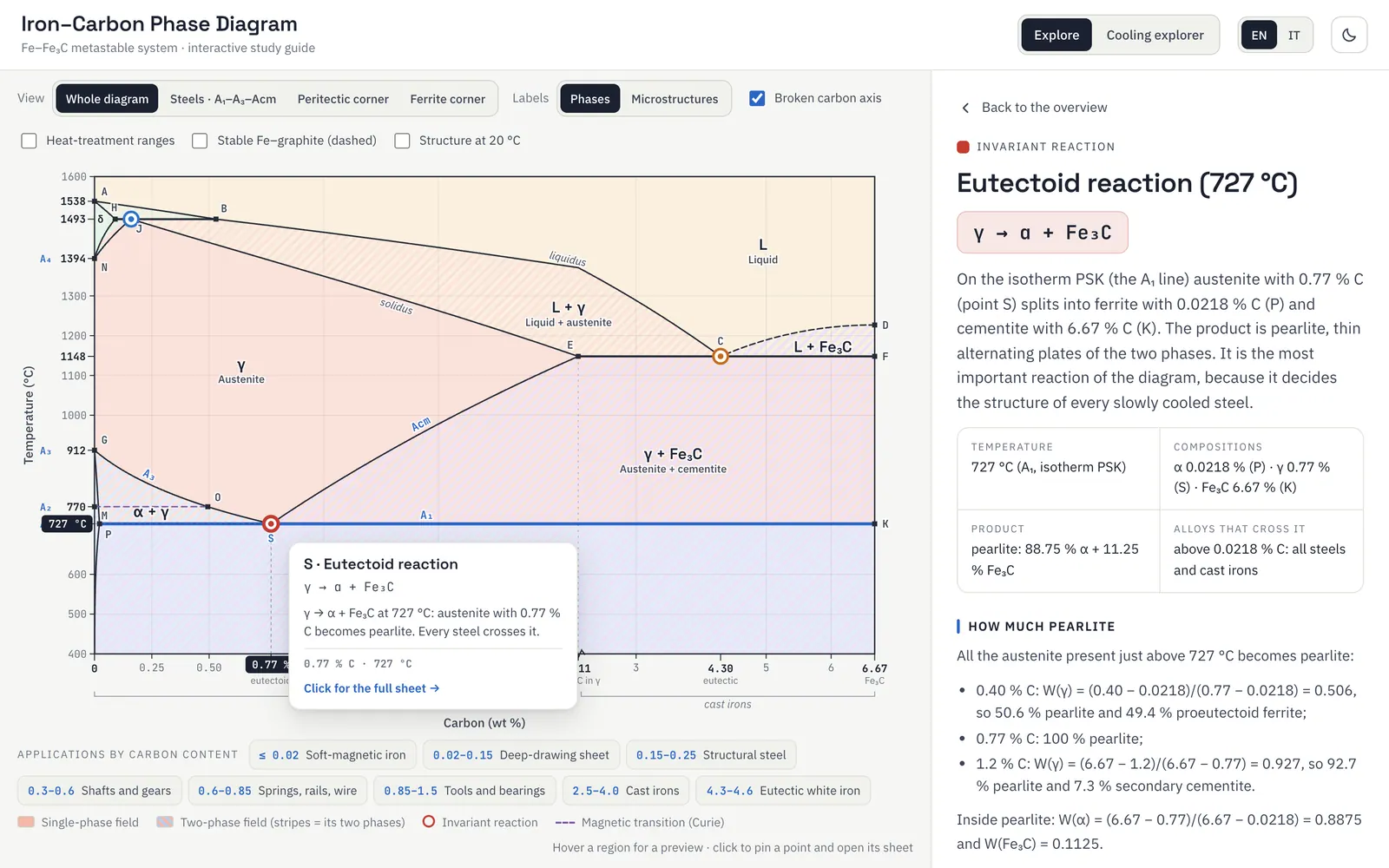
the eutectoid reaction at 727 °C, where austenite becomes pearlite
The diagram’s three invariant reactions sit on horizontal isotherms: the peritectic L + δ → γ at 1493 °C, the eutectic L → γ + Fe₃C at 1148 °C, and the eutectoid γ → α + Fe₃C at 727 °C, which is the one that governs every steel. The cooling path detects each of them at the exact temperature where it is crossed.
Checking the numbersLink to this section
I built the diagram on real numbers: the eutectoid at 727 °C and 0.77 % C, the eutectic at 1148 °C and 4.30 % C, the peritectic at 1493 °C, and cementite fixed at 6.67 % C. The curved boundaries between those points come from a thermodynamic (CALPHAD) calculation based on a published assessment of the Fe–C system (Gustafson, 1985), rescaled so that every line passes exactly through the textbook points.
One decision I'm particularly happy with is the carbon axis. Almost everything students work on sits between 0 and about 2 % C, the steel range, yet that's a thin slice of a diagram that runs all the way to 6.67 %. So I broke the axis. The steel range takes most of the width and stays readable, the cast-iron range is compressed, and a small break glyph tells the reader that the scale changes there.
LimitsLink to this section
It is a study aid to use next to the textbook. The diagram describes equilibrium, that is very slow cooling, so it says nothing about martensite or bainite. The cooling curve and the micrographs are schematic: they show the order of events, not real times or grain shapes. And real cast irons, which contain silicon, often follow the stable iron–graphite system, which the app only draws as a dashed overlay.