 Personal Project · Educational Tool
Frame Design: A Structural Solver Built for Students
A web tool for checking the beams, frames and trusses students practise on. Build the structure on a grid, press Solve, and read the reactions, the internal-force diagrams and a plain safety verdict. A trial version runs in the browser.
In short
- Problem
- Checking structural-mechanics exercises by hand is slow and error-prone, and professional solvers are built for engineers in industry, with a steep learning curve.
- Approach
- A deliberately narrow web tool. You build the structure on a grid and press Solve; a direct stiffness solver does the maths, and the design work goes into clarity and correct drawing conventions.
- Result
- Reactions, four diagrams (normal force, shear, bending moment, deflection), a one-line safety verdict with utilisation and deflection ratio, and a printable step-by-step solution.
- Tools
- React · SVG
You can try it here. This is a trial version: there is no account, and the structures you save stay in your browser.
Why I built itLink to this section
Many students find structural mechanics (scienza delle costruzioni) hard. Reactions, shear, bending moment, deflection: the theory is elegant, but the only way to own it is to solve problem after problem and check whether your answer is right. Checking by hand is slow, and it's easy to make mistakes.
Professional tools are powerful, but they are built for engineers in industry and come with a steep learning curve of their own. I kept thinking about the student who already struggles with the theory and is then asked to learn a complicated piece of software on top of it.
So I built Frame Design, a tool that checks the problems students practise on. Inside the app it is labelled Frame Solver. Most of those problems are statically determinate (isostatic) beams and frames from a first course, though the solver handles hyperstatic ones too. I kept the scope narrow on purpose, so the subject stays the hard part.
Less, but clearerLink to this section
I cut features hard and spent the complexity I saved on clarity. There is very little to configure and no manual to read. You open it, build the beam from your exercise, press one button and see whether it holds, and why.
So most of my time went into the experience around the maths: making structural analysis approachable enough that someone intimidated by the topic gets a result on the first try and, I hope, starts to enjoy it.
How it worksLink to this section
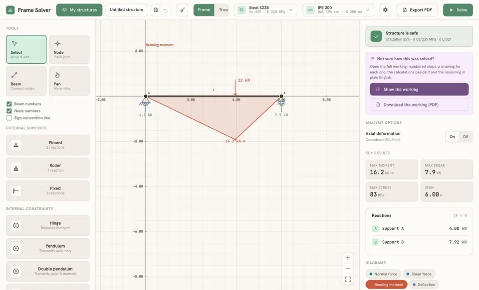
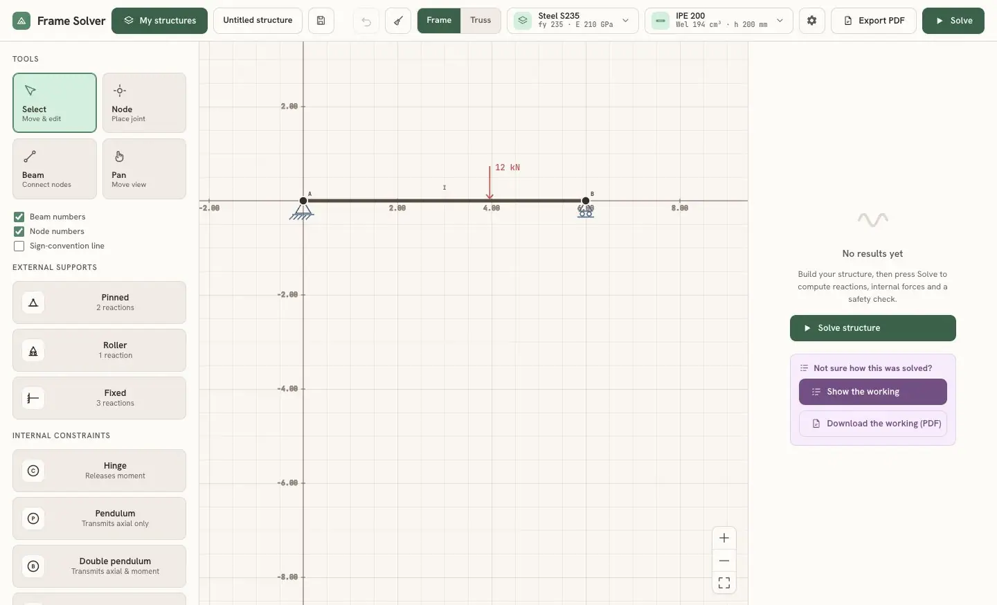
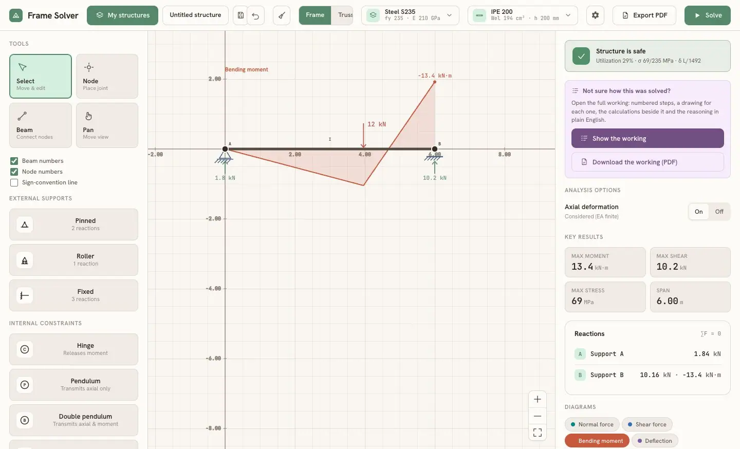
You work directly on a grid. Pick a tool, click to place nodes and join them into beams, then add the supports the problem calls for: pinned, roller or fixed, at any angle. Internal constraints go on the nodes too: a hinge, a pendulum, a double pendulum or a double-double pendulum. Loads can be point forces, distributed loads normal to the beam, linear loads in a global direction, applied moments or temperature changes. A switch in the top bar chooses the analysis model: Frame, where beams carry bending, or Truss, where every member is a pin-jointed bar.
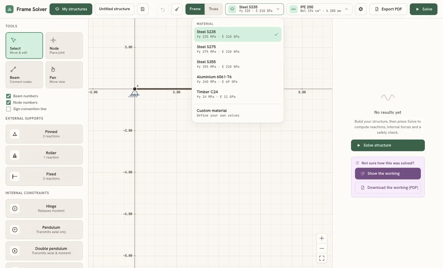
Every element is editable. Select it and a side panel lets you change its magnitude, position and direction. The material comes from a small library (Steel S235 / S275 / S355, Aluminium 6061-T6, Timber C24) or you define your own yield strength and elastic modulus, the way a textbook problem might give them. The cross-section works the same way: an IPE, HEA or HEB profile from the list, or a custom rectangle, circle or tube.
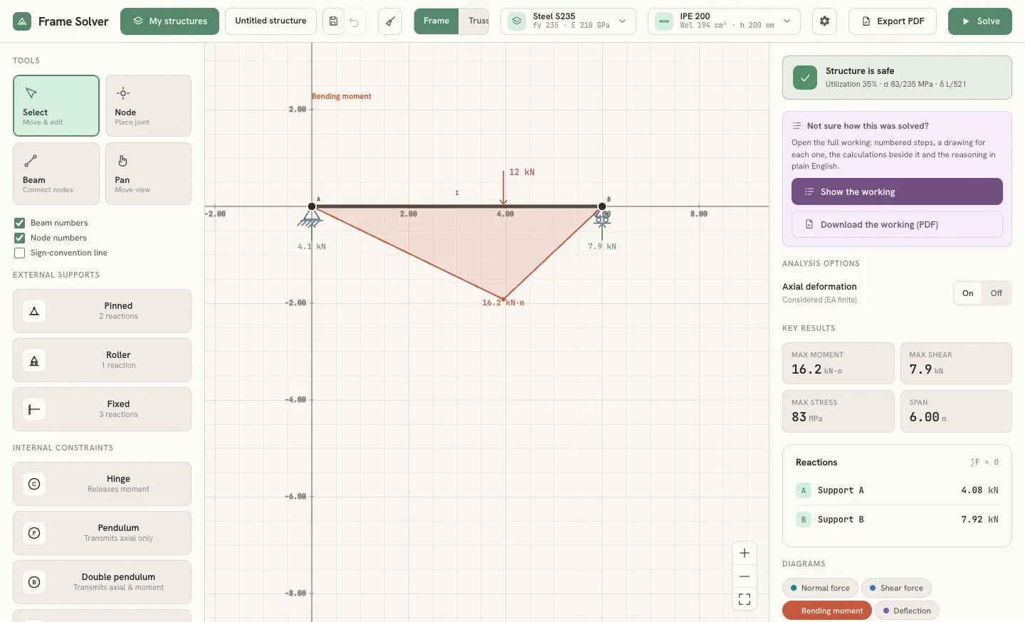
Press Solve and you get the support reactions, four diagrams (normal force, shear, bending moment and deflection) and a plain answer to is the structure safe? The tool compares the peak stress with the material's yield strength, reports a utilisation percentage and a deflection ratio, and puts the verdict in one line at the top of the results: green, amber above 80% utilisation, red when the section is overstressed.
what Solve computes for this beam: the free displacements, from the stiffness of the whole structure
Then every element gets its end forces back, and the reactions, the diagrams and the verdict all come from those numbers. The steps are explained below, under “How it solves a structure”.
The same button solves a hyperstatic structure. Turn the roller at B into a fixed support and the beam becomes a propped cantilever: the fixed end now takes a moment, and the reactions change accordingly.
How it solves a structureLink to this section
Under the Solve button there is one method: the displacement method in matrix form, usually called the direct stiffness method. Isostatic and hyperstatic structures go through exactly the same code. The solver never has to decide which redundant to remove or which compatibility equation to write, so a hyperstatic structure costs it no more work than an isostatic one.
The idea: unknown displacements instead of unknown forcesLink to this section
A frame is a set of straight elements joined at nodes. In the plane every node can move in two directions and rotate, so it has three degrees of freedom: u, v and θ. If I know how the two ends of an element move, I know the forces at its ends: that relation is the element's stiffness. So the unknowns become the displacements of the nodes, and the equations are the equilibrium of each node. A structure with j nodes gives 3j equations in 3j unknowns.
Compatibility comes for free, because two elements that share a node share its displacements. This is the opposite of the force method from the structural mechanics course, where you pick the redundants by hand and then write one compatibility equation for each.
1 · The element in its own axesLink to this section
Each element is an Euler-Bernoulli beam-column with six degrees of freedom, three per end, measured in the element's own axes (x along the element). Its 6×6 stiffness matrix is the textbook one. These are the same five terms the code builds, with the same letter names:
| a | 0 | 0 | −a | 0 | 0 |
| 0 | b | d | 0 | −b | d |
| 0 | d | e | 0 | −d | f |
| −a | 0 | 0 | a | 0 | 0 |
| 0 | −b | −d | 0 | b | −d |
| 0 | d | f | 0 | −d | e |
local stiffness matrix of a beam element · DOFs u₁ v₁ θ₁ u₂ v₂ θ₂
a = EA/L, b = 12EI/L³, d = 6EI/L², e = 4EI/L, f = 2EI/L. In truss mode every member is a pin-jointed bar and only the four a-terms survive.
2 · From the element's axes to the global axesLink to this section
An inclined element sees the world rotated by its angle α. The rotation matrix T turns global displacements into local ones, and the element's stiffness in global axes is TTkT. The rotation θ is the same in both frames, which is why the 1s on the diagonal stay put.
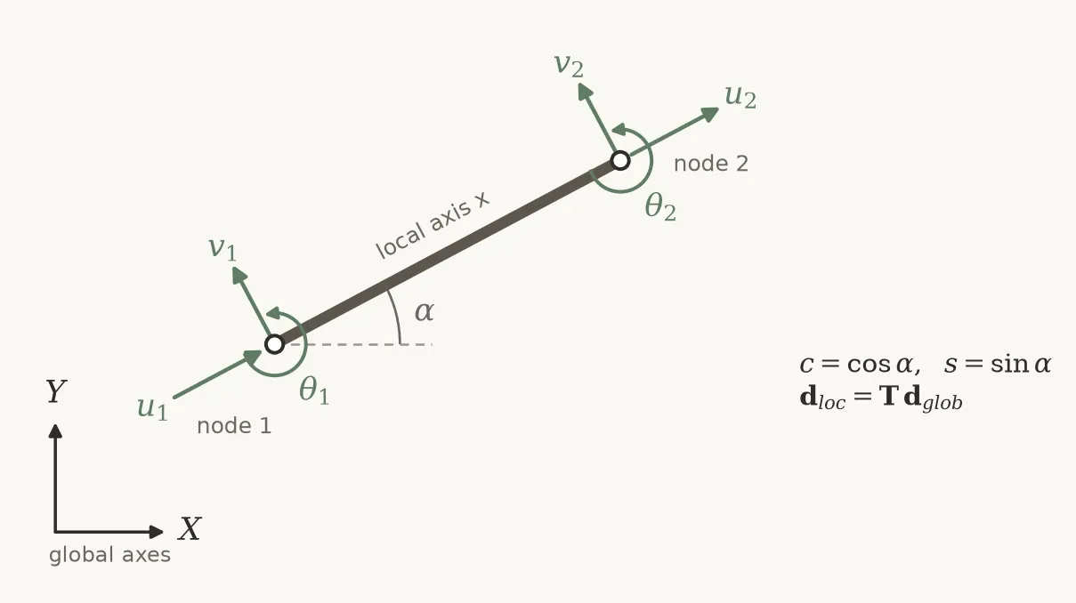
| c | s | 0 | 0 | 0 | 0 |
| −s | c | 0 | 0 | 0 | 0 |
| 0 | 0 | 1 | 0 | 0 | 0 |
| 0 | 0 | 0 | c | s | 0 |
| 0 | 0 | 0 | −s | c | 0 |
| 0 | 0 | 0 | 0 | 0 | 1 |
rotation matrix and element stiffness in global axes
c = cos α, s = sin α.
3 · The position matrices: putting every element in its placeLink to this section
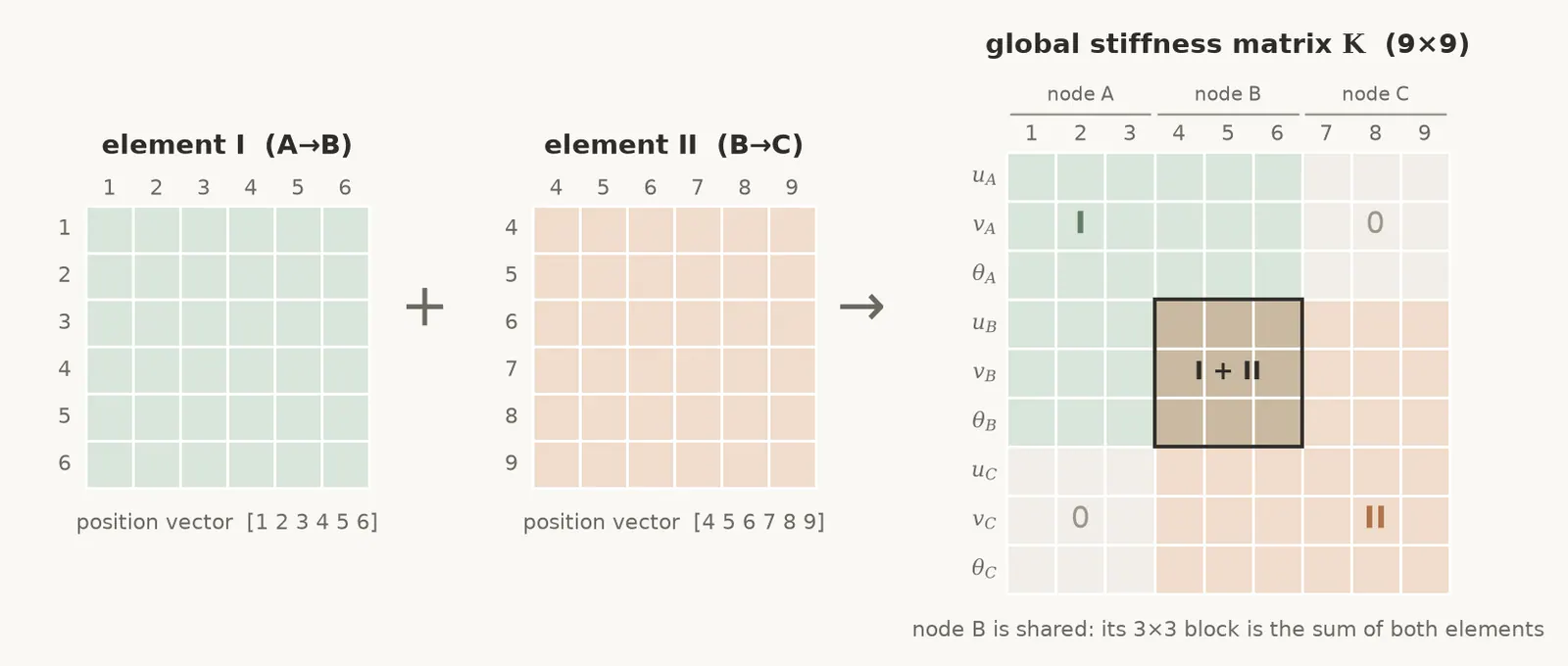
Every node has a number, and its three degrees of freedom occupy three fixed places in the global displacement vector. Element I, from node A to node B, therefore "lives" at positions 1 to 6 of the global vector, and element II, from B to C, at positions 4 to 9.
On paper this is written with a position matrix (books also call it the localization or connectivity matrix): a matrix of zeros and ones, Ae, that picks the element's six displacements out of the global vector. The global stiffness matrix is the sum of every element's contribution, each one moved into place by its own Ae:
| I | 0 | 0 |
| 0 | I | 0 |
| 0 | I | 0 |
| 0 | 0 | I |
position matrices and assembly · three nodes A, B, C, 3×3 blocks
I is the 3×3 identity and 0 a 3×3 block of zeros. dₑ = Aₑ d picks the element's six displacements out of the nine global ones.
Multiplying out all those zeros would be a waste, so the code keeps only what the matrix encodes: the list of six positions of each element, [3n₁, 3n₁+1, 3n₁+2, 3n₂, 3n₂+1, 3n₂+2], where n₁ and n₂ are the numbers of its two nodes counted from zero, and adds every term of kg straight into its row and column of K. Where two elements meet, their terms add up, and that sum is the equilibrium of the shared node written in matrix form.
4 · Loads along a member become loads at the nodesLink to this section
The stiffness method only accepts forces applied at nodes. A load acting along an element is replaced by its equivalent nodal loads, the work-equivalent forces computed with the same cubic shape functions that describe the element's deflection. For a uniform load q on an element of length L:
equivalent nodal loads of a uniform load, local axes
These are the classical fixed-end forces with the sign reversed. Point loads use the shape functions at the load position; distributed and trapezoidal loads are integrated numerically in 80 strips; couples and thermal loads (N = EAαΔT, M = EIα(T_bottom − T_top)/h) have their own terms.
5 · Supports, then solvingLink to this section
A support blocks some of the node's degrees of freedom: a pin blocks u and v, a roller blocks one translation, a fixed support blocks all three. Splitting the degrees of freedom into free (f) and constrained (c) ones, the system becomes:
| Kff | Kfc |
| Kcf | Kcc |
| df |
| 0 |
| Ff |
| Fc + R |
partitioning: only the free rows are solved
The support displacements are zero, so the free displacements come from the first block row alone.
In the code the constrained rows and columns are zeroed with a 1 on the diagonal, which gives the same solution without reshuffling the matrix. The generated report (step 4 below) describes this step as removing those rows and columns; the two are equivalent. A roller at an arbitrary angle cannot be expressed as a blocked u or v, so it gets a very stiff spring along the blocked direction (a penalty, 10⁸ times the largest of EA and EI). The system is solved by Gauss-Jordan elimination with partial pivoting, and a pivot counts as zero below a tolerance scaled on the stiffness of the structure, not a fixed small number.
One more check catches mechanisms. When the structure is a mechanism the matrix is singular, and the elimination can still return a displacement field that means nothing. So after solving, the code plugs the displacements back into the original equations on every free degree of freedom. If the residual is larger than 0.1% of the largest nodal load, it refuses the result and says the structure is a mechanism.
6 · Back to the elementsLink to this section
With the nodal displacements known, each element gets its end forces back through the same position vector and rotation:
end forces of each element, local axes
Everything else comes from those six numbers per element. The reactions are the end forces summed at each supported node and turned back into global axes. N, V and M along the element follow from the end forces plus whatever load lies between the end and the cut, sampled at 101 points per element. The deflection is the curvature M/EI integrated twice along the element, starting from the displacement and rotation of its first node, with a linear correction so that it lands exactly on the displacement of the second.
Internal hinges and other internal constraintsLink to this section
An internal hinge does not add a node or a degree of freedom. The node keeps its single rotation. Of the element ends that meet at the hinge, one stays rigid and carries that rotation, and the others are "released": their end moment is forced to zero by static condensation of the element matrix before assembly. If a continuous beam passes through the node, only the members resting on it are released. The same trick covers the other internal constraints, which release different components: a pendulum (V and M), a double pendulum (V) and a double-double pendulum (N and V).
static condensation of the released degrees of freedom c (r = retained)
The condensed matrix and load vector replace k and f, so the released end transmits no force in that component.
A beam drawn straight across a support or across the end of another beam is split there automatically, so the two actually connect.
Isostatic or hyperstatic?Link to this section
The solver handles both the same way. For a student the distinction matters, so the step-by-step report starts by counting:
degree of static indeterminacy
m members, r reaction components, j nodes, s released internal conditions. For a truss: i = m + r − 2j. i = 0 is isostatic, i > 0 hyperstatic, i < 0 a mechanism.
When the equilibrium of the whole structure is enough to fix the reactions (an isostatic structure without internal hinges), the report finds them the way you would by hand: one equilibrium equation at a time, taking moments about each support, and then checks them against the stiffness solution. Otherwise, as in a hyperstatic beam or a three-hinged frame, it takes the reactions from the stiffness solution and uses the equilibrium equations as a check.
A worked example: a two-span continuous beamLink to this section
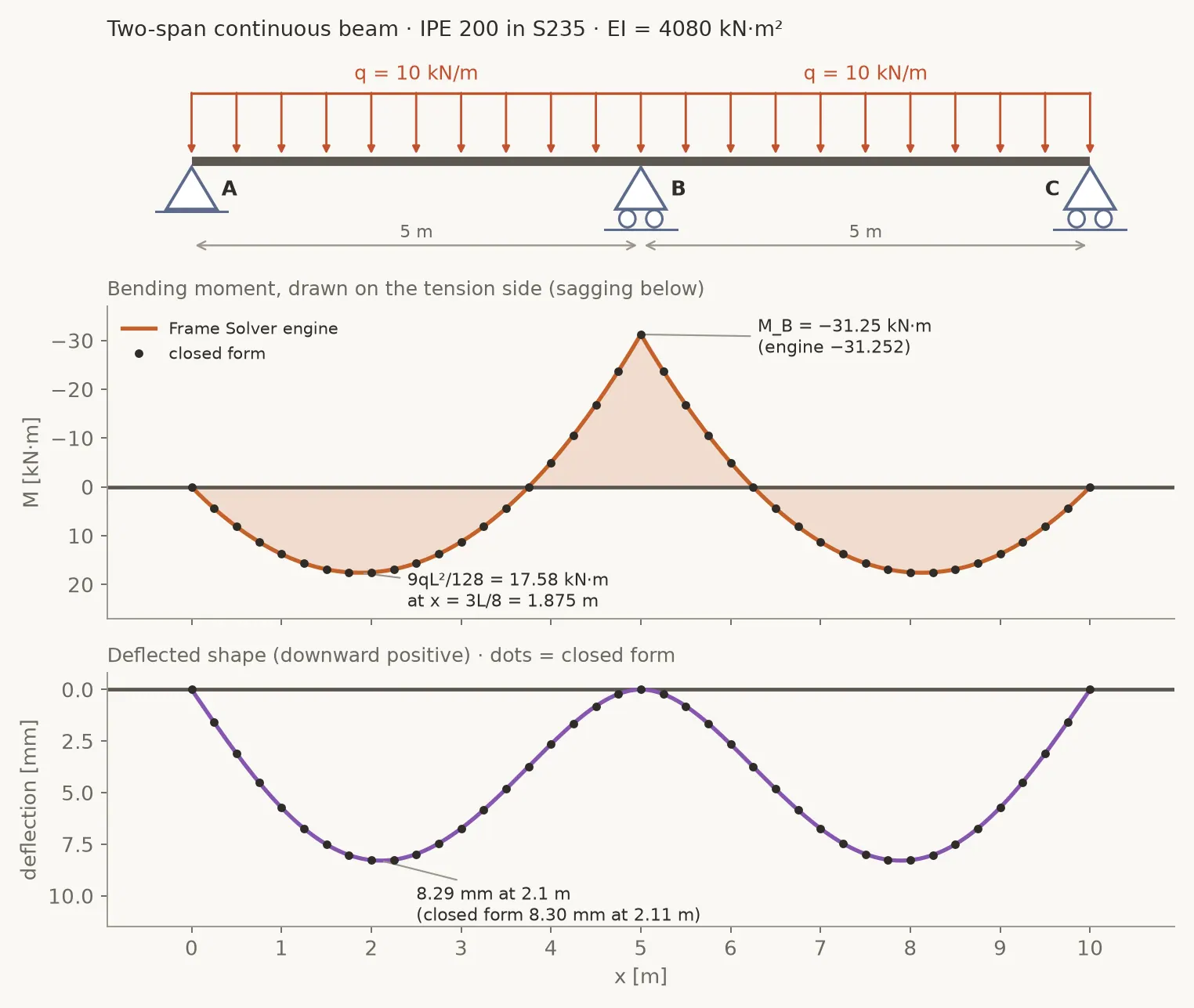
To check the engine I ran the classic hyperstatic beam through it: two spans of 5 m, a pin at A, rollers at B and C, a uniform load of 10 kN/m over the whole length, an IPE 200 in S235. That gives EI = 210 000 MPa × 1943 cm⁴ = 4080.3 kN·m², and the count is i = 3·2 + 4 − 3·3 − 0 = 1: hyperstatic once.
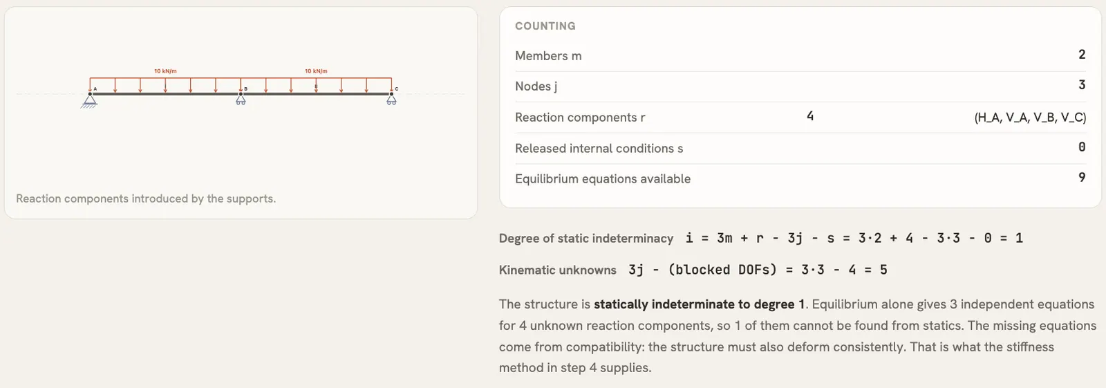
The global matrix is 9×9. The supports block four degrees of freedom (uA, vA, vB, vC). Of the five free ones, the two axial displacements carry no load and come out zero, so the problem reduces to the three rotations. Node B appears in both elements, so the position matrices add its two contributions on the diagonal: 4EI/L + 4EI/L = 8EI/L.
| 4 | 2 | 0 |
| 2 | 8 | 2 |
| 0 | 2 | 4 |
| θA |
| θB |
| θC |
| −20.835 |
| 0 |
| +20.835 |
reduced system, rotations only · numbers from the engine (kN·m, rad)
The right-hand side is ∓qL²/12. The engine gets 20.835 instead of 20.833 because it integrates the distributed load numerically; this 0.008% is behind the small differences in the reactions and in the moment over B.
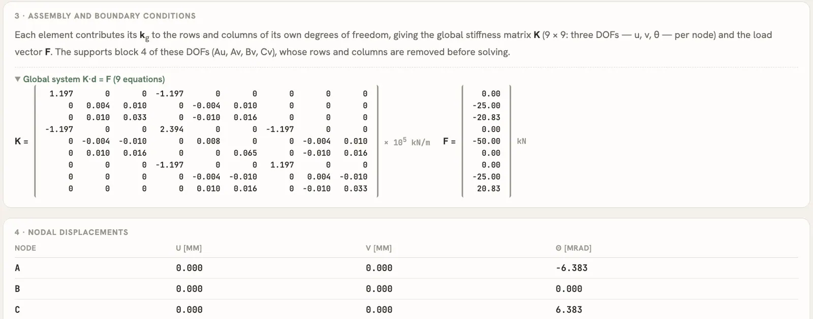
From the rotations, the end forces of element I give the moment over the middle support: MB = 2EI/L · θA − qL²/12 = 1632.1 · (−6.3828·10⁻³) − 20.835 = −31.25 kN·m. Here is the engine next to the textbook formulas:
| Quantity | Engine | Closed form | Value |
|---|---|---|---|
| Reactions at A and C | 18.750 kN | 3qL/8 | 18.750 kN |
| Reaction at B | 62.501 kN | 5qL/4 | 62.500 kN |
| Moment over B | −31.252 kN·m | −qL²/8 | −31.250 kN·m |
| Largest sagging moment | 17.574 kN·m (diagram sampled every 5 cm) | 9qL²/128 at 3L/8 | 17.578 kN·m at 1.875 m |
| Rotation at A | −6.3828·10⁻³ rad | −qL³/(48EI) | −6.3823·10⁻³ rad |
| Largest deflection | 8.292 mm at 2.10 m | 0.005416 qL⁴/EI at 0.4215 L | 8.296 mm at 2.11 m |
The differences are all below 0.06%, and they come from three places: the numerical integration of the distributed load, the 5 cm sampling of the diagrams and, for the deflection, the step-by-step integration of the curvature. The report's own per-segment equation puts the largest sagging moment at 17.58 kN·m at x = 1.875 m.
What the student sees: "Show the working"Link to this section
All of this would stay hidden behind the Solve button, so I built a second button. "Show the working" opens a separate, printable page that walks through the solution of whatever structure is on the canvas, in seven numbered steps:
- The model: nodes, members, supports, loads, material and section.
- Static classification: the count above and what it means for the method.
- Support reactions: loads reduced to resultants and global equilibrium, solved one unknown at a time when global equilibrium alone is enough.
- The stiffness solution: element matrices k, T and kg, the equivalent nodal loads of each loaded element, the assembled K and F, the blocked degrees of freedom, the nodal displacements and the end forces.
- Internal forces, element by element: N(x), V(x) and M(x) as equations for each segment, with the point of zero shear and the local extreme of M. For a truss this becomes the method of joints.
- Diagrams: N, V, M and the deflected shape, drawn as on the canvas.
- Verification: the stress and deflection check.
Two rules shaped it. First, every number on that page comes from the same solver that draws the diagrams, run once more with every intermediate quantity kept; nothing is re-solved with a second implementation that could disagree. Second, where I show a hand derivation (global equilibrium, the N/V/M equations of a member), it is derived independently and then compared with the solver, and the page prints the result of that comparison. Hovering over a load or a support highlights the lines of calculation that use it.
Getting the details rightLink to this section
A student can't tell when a solver is slightly wrong, so I spent a lot of time on conventions.
The diagrams follow the structural drawing convention: the bending moment is drawn on the tension side, so a sagging, gravity-loaded beam shows its moment below the axis, while shear stays above.
Then there was scale. At first every force arrow and every diagram was drawn at a fixed size, which hid the magnitudes. Now arrows and distributed loads grow with the load, scaled to the largest load on the structure, so a bigger force always looks bigger. Diagrams in the same unit share one scale, so you can compare their sizes straight off the screen, as you would on paper.
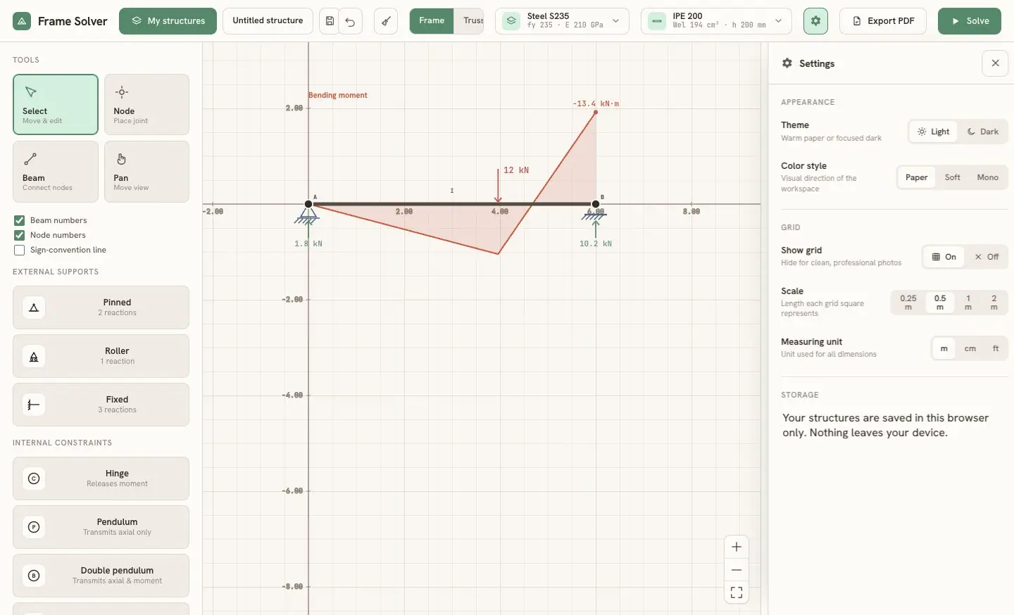
There were smaller fixes too: rotation handles that turn the way your hand expects, and a settings panel for theme, grid scale and units (metres, centimetres or feet).
LimitsLink to this section
- The analysis is plane, linear and limited to small displacements. K is built once on the undeformed geometry, so there is no geometric nonlinearity and no buckling. The elements are Euler-Bernoulli, so shear deformation is ignored.
- There is one material and one section for the whole structure: every element uses the same E, A and I.
- There are no elastic springs and no imposed settlements. The supports are rigid; only inclined rollers use a penalty spring internally.
- The option to neglect axial deformation is an approximation: it multiplies EA by 10⁴ instead of imposing exact constraints.
- The safety check is simple. It compares Mmax/Wel (or N/A in a truss) with the yield strength: no partial safety factors, no N+M interaction, no buckling. The report says so on the page.
- The solver works on a dense 3j × 3j matrix, which is fine for exercise-sized structures and not meant for large models.
- Two things are still on my list: the deflection ratio divides by the total length of all members, which flatters a multi-span beam (the example shows L/1206 instead of L/603 per span), and the report prints "x^1" where it should print "x".